The A* pathfinding algorithm is designed to find the shortest path between two vertices on a graph.

It’s an enhancement of Dijkstra’s algorithm, but, potentially much more efficient. Dikstra’s algorithm will find the shortest path from a given vertex to ALL of the other vertices in a graph. But this may be more information than we need, and therefore more work than we need to do.

If all we’re interested in is the shortest path between TWO particular vertices, then the A* algorithm is a better choice.

The A* algorithm, and its numerous variations, is widely used in games programming, natural language processing, financial trading systems, town planning and even space exploration.

Heuristics

Consider the following undirected, weighted graph:

 

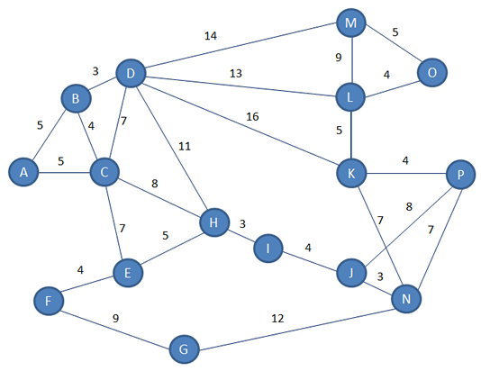
The information you can see here is crucial, but it’s not enough for A* to work. We need more information than this.

The A* algorithm depends on so called heuristic estimates. A heuristic estimate is basically an educated guess. Each time we move from one vertex to another, we need an estimate of the remaining distance to the destination. This estimate will inform the next move.

The A* algorithm might not work efficiently if we seriously underestimate the remaining distance, and it might not work at all if we over estimate it. We say that our heuristic should be admissible.

This means we need some extra information about each vertex, so that we can
calculate these estimates. In a system where the vertices are geographical locations on a map, and the edges are distances in kilometres for example, we might know the longitude and latitude of each vertex, so we can calculate the straight line distance from any location to the destination.

Another way is to use grid coordinates to describe the location of each vertex. If we were implementing this with an object oriented approach, then each vertex could store its own X and Y coordinates.

So, suppose we wanted to estimate the remaining distance from E to P.

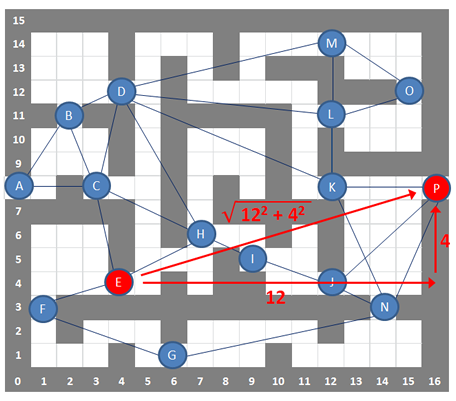
Ignoring any obstacles, we could move 12 steps to the right, then 4 steps upwards. If we wanted to, we could then use Pythagoras’s theorem to calculate the Euclidean distance, that is, the straight line distance between E and P.

Alternatively, we could simply use the total number of steps, namely 12 + 4 = 16. This, after all, is just an estimate. On a grid system like this, this is known as the Manhattan distance. If you have ever been to New York in the USA you’ll know that the streets are laid out in strict rectangular blocks and getting from one place to another is pretty much like this.

A* Walkthrough

We want to find the shortest path from A to P. A table can be used to record the results of our calculations.

The heuristic distance from each vertex to the destination, that is, the so called h value, has been pre-calculated, based on information we already have. We’ve used the grid coordinates of each vertex to calculate its Manhattan distance to the P. These h values have been calculated in advance, but the truth is, they don’t need to be. If things go well, we’re not going to need all of them, so it’s possible that a program would calculate them as and when it needs them.

We maintain two lists. One of open vertices, and one of closed vertices. We begin by adding our starting vertex A, to a list of open vertices, then A becomes the current vertex.

Next we need to calculate the g value of vertex A. The g value of a vertex is the distance travelled from the start to get to it. The distance from A to A is obviously 0.

The g value for A is then added to the heuristic distance from A to P, the so called h value, and this gives us an f value of 0 + 16. That is, 16.

Now we add any vertices that are adjacent to the current vertex to the list of open vertices, in this case B and C, and we calculate their f values, by adding their distances from A to their h values. We also make a note of the vertex we came through to get to each of these, in the previous vertex column.

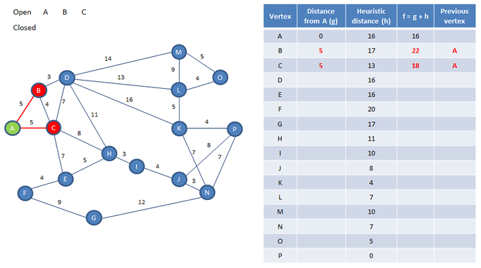
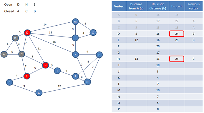
Now we can add vertex A to the list of closed vertices. Our next job is to select a new current vertex from the list of open vertices. The most promising one is the one with the lowest f value. We can see from the table that in this case its vertex C, so C becomes the new current vertex.

Now we add the vertices connected directly to C to the open list. We need their f values.

These open vertices are known as the fringe, or the frontier.

One of these will become the successor to C, one of these will be the next current
vertex.

One vertex at a time, we calculate its g value followed by its f value. Each g value is the g value of the current vertex, which we can read straight from the table, plus the extra distance to the potential successor.

Notice that we calculate a new g value for B even though it has one already, it too is a potential successor to C. For all we know, it may be quicker to get from A to B via C, rather than by taking the direct route.

You can see here though that the alternative f value for B is bigger than the previous one, so this doesn’t appear to be a better path to explore. The alternative f value for B is therefore ignored. If the new value has been smaller, the existing g and f values would have been replaced.

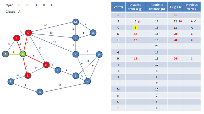
Now we can now close C, and choose its successor; the one with the smallest f value.

The process continues. When choosing the next current vertex, if we have more than one open vertex with the same lowest f value, any one of them can be selected arbitrarily.

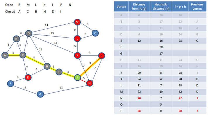
Eventually, the destination vertex will be opened, but the search is not necessarily over. Its f value should be calculated and only if it is the lowest of the open vertices can we be reasonably sure that we have found the shortest path – maybe!

The g value of P, gives us the path distance we are looking for, and since each vertex has a record of the vertex that came before it, we can trace these backwards to get the path sequence we have been looking for.

Features of A*

• A* has a wide range of applications
• A* finds the shortest path between two vertices
• A* does not have to visit all vertices, ideally
• A* picks the most promising looking node next
• The better the heuristic, the quicker A* finds the path
• Heuristic is problem specific
• Open nodes known as ‘the fringe’ or ‘the frontier’
• List of open nodes can be implemented as a priority queue
• Each node on the path keeps track of the one that came before it
• A* will always find a solution if one exists

With A* we don’t necessarily need to visit every single vertex in the graph. You can imagine that with a much bigger graph, with a lot more vertices involved, there would be a larger proportion of unopened vertices.

There is another path in this graph which also has a distance of 28 that we might have found instead. At an early stage in the process with this graph, we had to choose which of D or H should be the next current vertex. In this walkthrough H was chosen, and that influenced the course of events that followed. In fact, we had another arbitrary choice to make near the end of the process, and decided to make J current, and arguably we got lucky. A different choice would have slowed things down for sure.

This tells us something important about A*; It’s guaranteed to find a path, if a path exists, but how quickly it does so, depends to some extent on chance, but very much on the quality of our heuristics. Ideally, the heuristic estimates of the remaining distances should be as close as possible to the actual remaining distances, but not greater. If these estimates are too small, the frontier will expand unnecessarily, and more time will be spent barking up the wrong tree. In fact, if the heuristics were all zero, every vertex in the graph would have been be explored – which is exactly what Dijkstra’s algorithm does. If the heuristics are overestimated on the other hand, A* will find a path if it exists, but it may not be the shortest path.

Of course, calculating the best possible heuristic estimates, is easier said than done. What if our graph represented a magical maze with features like inter-dimensional gateways, deadly swamps, fiery larva pits, or teleporters. Then the costs of the edges of the graph would bear little relationship to physical space, and using the Manhattan distance as the basis for heuristic calculations would be nonsense. The choice if heuristic depends very much on the nature of the nature of the
problem.

Pseudocode

 

Initialise open and closed lists
Make the start vertex current
Calculate heuristic distance of start vertex to destination (h)
Calculate f value for start vertex (f = g + h, where g = 0)
WHILE current vertex is not the destination
     FOR each vertex adjacent to current
         IF vertex not in closed list and not in open list THEN
             Add vertex to open list
         END IF
         Calculate distance from start (g)
         Calculate heuristic distance to destination (h)
         Calculate f value (f = g + h)
         IF new f value < existing f value or there is no existing f value THEN
             Update f value
             Set parent to be the current vertex
         END IF
     NEXT adjacent vertex
     Add current vertex to closed list
     Remove vertex with lowest f value from open list and make it current
END WHILE