Searching a graph

Searching a graph involves systematically visiting and testing each vertex in the graph to see if it is the target vertex.  There are two ways to traverse a graph.  These are depth first and breadth first.

NOTE:
A tree data structure in which a node can have several child nodes (i.e. not a binary tree), is actually a special type of graph (i.e. a graph with no cycles), so the traversal methods described here apply to it.  However, The recursive depth first traversal methods used for a binary tree (pre-order, in-order, post-order) do not apply to graphs.

Depth first traversal

Depth-first search involves following a path from the starting vertex until the last vertex on that path is reached.  We then backtrack and follow the next path until the last vertex on that path is reached.  This process continues until there are no more paths left to explore.  Depth first traversal and back-tracking can be achieved by using a stack data structure.

Depth first traversal algorithm

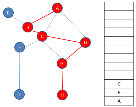
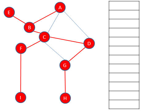
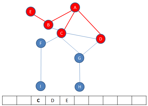
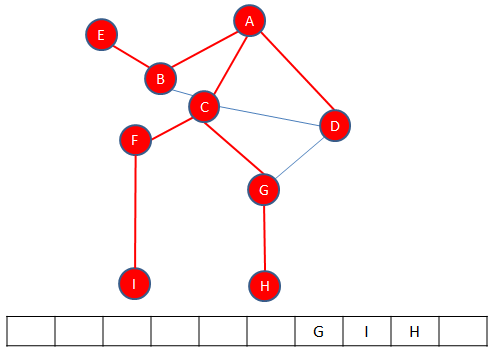
First, the starting vertex is visited, which can actually be any vertex.  The starting vertex on the graph below is A.  Vertex A is pushed onto a stack and the fact that it has been visited is recorded somehow.  Then, an unvisited vertex adjacent to A is selected and visited, in this example B is selected.  Vertex B is also pushed onto the stack and the fact that it has been visited is also recorded. Then, an unvisited vertex adjacent to B is selected and visited, in this case C is selected.  Vertex C is pushed onto the stack and the fact that it has been visited is recorded. This process continues until the last vertex along a particular path is reached, in this case H.  Exactly which path is followed to begin with is not particularly important, that will depend on the decisions made when the algorithm is implemented.  What matters is that the algorithm drills down one particular path as far as it can go.

 

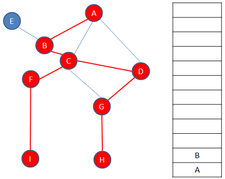
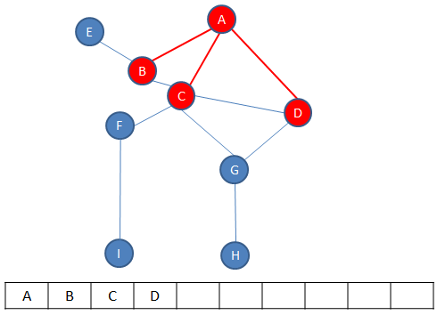
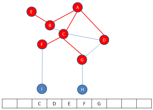
Each time a vertex is pushed onto the stack, a check is made to see if it has any unvisited adjacent vertices.  If it doesn’t have any, the path must be exhausted and it’s time to backtrack.  A vertex without unvisited adjacent vertices is popped off the top of the stack.  The new top vertex is then checked for unvisited adjacent vertices.  If it has none, it too is popped off the top of the stack and the new top vertex is checked in the same way.  This continues until there is a vertex at the top of the stack with unvisited neighbours.  This means there is another path to explore.  In this example, C finds itself at the top of the stack.

,

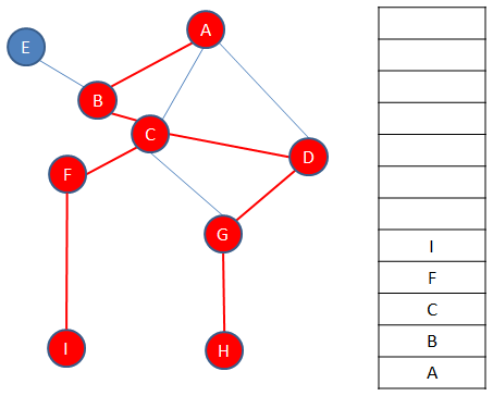
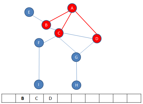
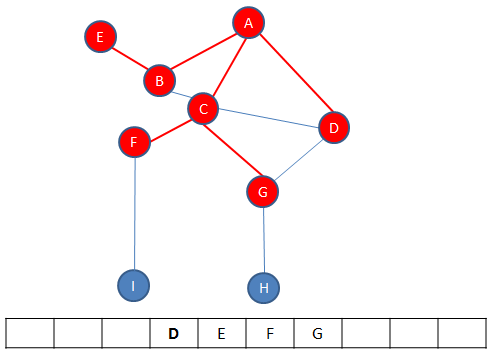
Once again, vertices are pushed onto the stack as a new path is explored, in this example vertex F then vertex I, until there are no more unvisited vertices on that path.

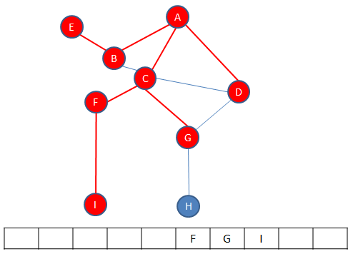
When the next path is exhausted, it is time to backtrack again to a vertex with unvisitied neighbours, in this case to vertex B.

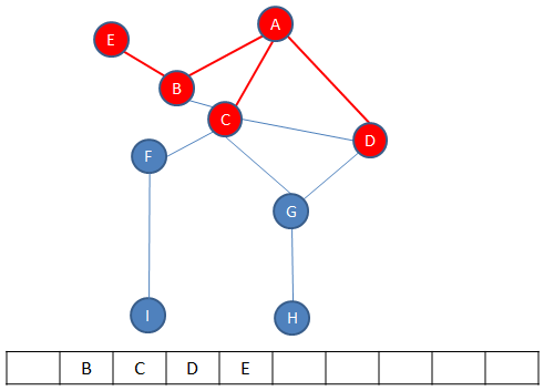
There is another path to explore, which ends with vertex E.

Backtracking from E, brings us back to A, and there are no more paths to explore.  The traversal is complete.

Here is the depth first traversal algorithm expressed in words.

Push the first vertex onto the stack

Mark this vertex as visited

Repeat

        Visit the next vertex adjacent to the one on top of the stack

        Push this vertex onto the stack

        Mark this vertex as visited

        If there isn’t a vertex to visit

              Pop this vertex off the stack

        End if

Until the stack is empty

Note that much of the implementation detail is missing from the algorithm above.  For example, to implement this you need some system for ‘marking’ a vertex as visited.  This might mean having a ‘Visited’ property of the Vertex class if you are taking an OOP approach.  Alternatively, you could maintain an array of visited vertices.  Furthermore selecting the next adjacent vertex means examining the edge data in the graph’s adjacency matrix.

Breadth first traversal

Breadth-first traversal starts at the first vertex and tries to visit all of the vertices as close to the this vertex as possible. We are effectively moving through a graph layer by layer, first examining the layers closer to the first vertex and then moving down to the layers furthest away from the starting vertex.  This can be achieved using a queue data structure.

Breadth first traversal algorithm

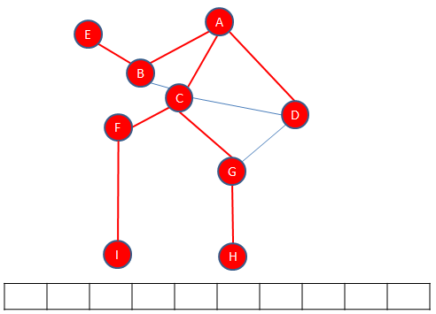
The start vertex, in the case A is enqueued. Then each of its adjacent vertices are enqueued.

Then A is dequeued, leaving B at the front.

Now all of the neighbours of B are enqueued.  In this case there is only E.

B is dequeued, leaving C at the front.

The neighbours of C are enqueued.

C is dequeued leaving D at the front.

D has no unvisited neighbours so it can be dequeued immediately.  E is then at the front but it too has no unvisited neighbours so is dequeued immediately, leaving F at the front.

 

The only unvisited neighbour of F, namely I, is enqueued.

F is dequeued, so G is at the front.

H is enqueued.

G is dequeued, so is I and so is H.  An empty queue indicates that the traversal is complete.

Here is the breadth first traversal algorithm expressed in words.

Enqueue the first vertex

Mark the first vertex as visited

Repeat

        Visit next vertex adjacent to the first vertex

        Mark this vertex as visited

        Enqueue this vertex

Until all adjacent vertices visited

Repeat

        Dequeue next vertex from the queue

        Repeat

               Visit next unvisited vertex adjacent to that at the front of the queue

               Mark this vertex as visited

               Enqueue this vertex

        Until all adjacent vertices visited

 Until the queue is empty